Traditional OLAP database execution engines were designed for the CPU: 1) optimized for a handful of powerful cores, 2) deep cache hierarchies, and 3) sequential or lightly vectorized processing. In the past decade, however, GPU performance and functionality have greatly advanced, driven largely by the generative AI revolution, to the point of becoming a viable platform for running relational workloads. GPU-accelerated data systems that can run queries orders of magnitude faster than their CPU equivalents will enable the next big revolution in analytics, fuelled by AI agents. Their architecture and programming models are, however, different enough from the CPU, that specialized algorithms must be developed to achieve high performance on analytical workloads. This post aims to illuminate the kind of algorithms NVIDIA’s RAPIDS project has built to close that gap. It is the first in a series exploring libcudf, NVIDIA’s core DataFrame library for single-node GPU data processing.
TL;DR
- The post dives into libcudf's hash-aggregate fast path for a
GROUP BY … SUM query with low per-block key cardinality: each block must see at most 128 distinct grouping values to stay on the shared-memory path.
- For the dataset analysed, libcudf uses a two-level shared-memory strategy to tame atomic contention. Each CUDA block deduplicates its rows in a private on-chip hash set before touching global memory, so the device-wide hash set sees at most one insert/lookup per distinct key per block and the output column receives at most one atomic add per distinct key per block, not one per row.
- The algorithm runs in four sequential phases. (1) Initialize the device hash set with a sentinel value; (2) map every row to a block-local rank and elect cross-block key representatives via CAS into the device hash set; (3) retrieve unique keys from the hash set and rewrite index arrays to dense output offsets; (4) accumulate partial sums in a shared-memory accumulator array, then flush one atomic add per group per block to the output column.
- For 100M rows, the dominant cost is data structure overhead, not compute. A significant fraction of total kernel time is spent initialising the oversized hash table (allocated at 2× input size) and scanning it in the Interlude, costs that are independent of key cardinality and grow with input size. Future posts will explore performance at higher scale factors.
This report was produced with the help of AI agents.
1. Introduction: Relational Algebra on GPUs
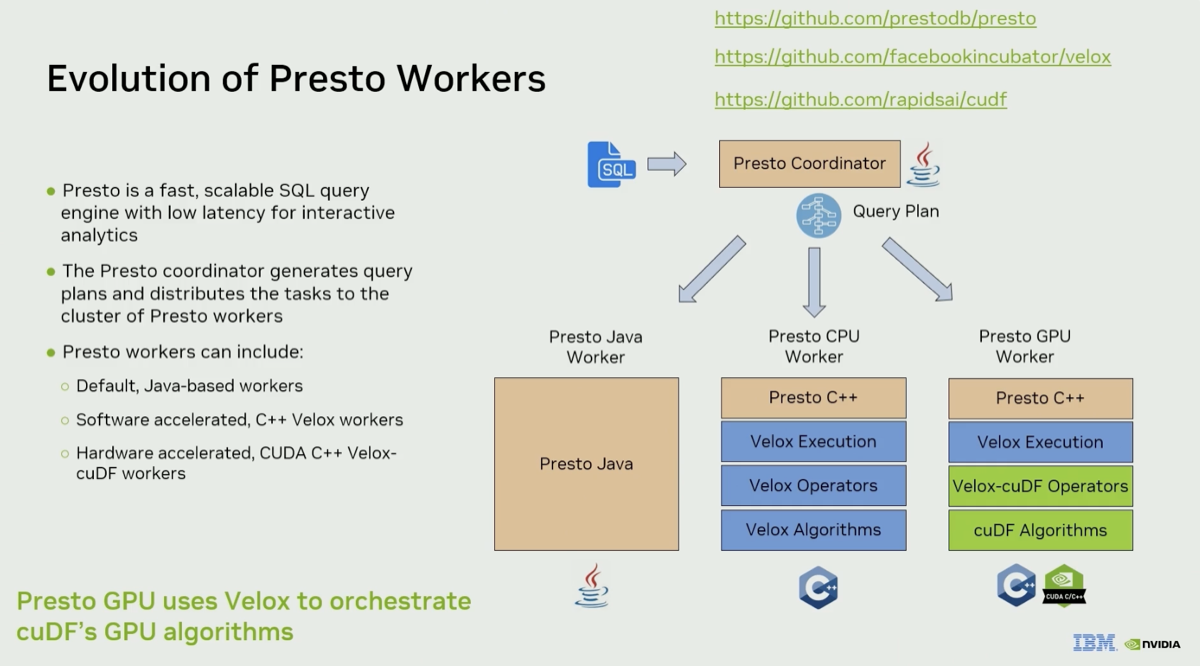
Mapping relational algebra onto GPUs introduces a massive semantic gap compared to CPU. Operators like joins, aggregations, and sorts must be entirely reimagined for the GPU SIMT (Single Instruction, Multiple Thread) architecture. Conventional algorithms natively optimized for CPUs often hit brutal bottlenecks on GPUs due to thread divergence, uncoalesced memory access, and severe penalties for global synchronisation.
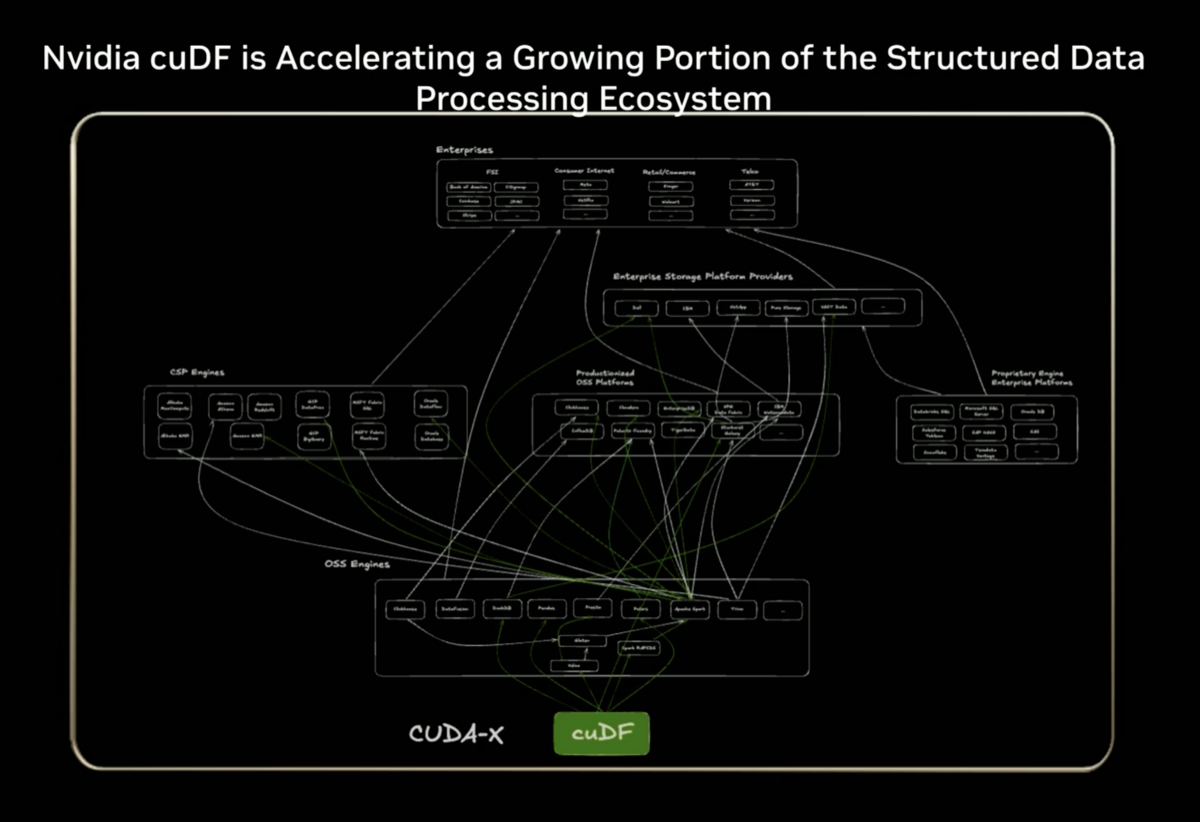
To bridge this runtime gap, NVIDIA developed libcudf: a C++ library implementing foundational DataFrame operations and relational primitives natively on the GPU. It has emerged as the de facto execution framework for a massive portion of the accelerated data ecosystem, underpinning projects like Spark RAPIDS, Dask-cuDF, Velox CuDF and numerous independent database research efforts.
The central questions driving this exploration are:
- How does libcudf translate fundamental relational operators into massively parallel GPU kernels?
- What are its structural strengths, and where does the GPU memory/compute model impose hard limits?
- What does the developer tooling look like, and how does one reason about its hardware utilization?
To answer these questions, I begin by identifying at a high level which algorithms underlie key primitives. I take as an example the simple groupby aggregation and break down into components showing how the library implements them. I identify the main data structures and provide illustration that show the movement of data as the algorithm runs. While some runtime info is provided for the 100M dataset in this post, the next one will focus on actual run and reviews learning from the debugging tools.
The Aggregation Problem
GROUP BY is one of the foundational operators in relational database systems. Its job is to partition an input relation into disjoint subsets then reduces each group to a single output row by applying one or more aggregate functions. For example, a simple question a retail merchant might ask is what the breakdown of the total price of orders by order status, identifying the amount of missed dollar opportunity for orders not completed and investigating improvements. We will use this example in the rest of the blog post.
In a query execution engine the GROUP BY physical operator must solve two logical subproblems:
-
Key partitioning: determine, for every input row, which output group it belongs to. This is effectively a dictionary-encoding problem: map an arbitrarily-typed key (integer, string, composite) to a dense integer group-id in [0, K) where K is the number of distinct keys.
-
Aggregation: reduce all rows assigned to the same group-id to a single scalar per aggregate column (e.g., sum all values from column C for group-id 3), using an aggregate function such as SUM, COUNT, MIN, MAX, AVG, etc
These two subproblems are algorithm-agnostic: the same logical goals can be achieved via two fundamentally different physical strategies.
- The sort-aggregate approach sorts all rows by key first, after which identical keys are contiguous and can be reduced in a single scan; comparison sort costs O(n log n), while radix sort can be linear for fixed-width keys.
- The hash-aggregate approach builds a hash table mapping each distinct key to its running accumulator, updating it in expected O(n) time, no sort required, but concurrent writes to shared buckets introduce contention.
The algorithm must also be adapted to the number of keys and columns being operated on as well as the kind of data types used for partition and aggregation. Simple primitive types like float and int come with hardware and basic language support, while more advanced ones like string and datetime require specialized handling.
Recently, a big use case has been supporting user-provided functions (UDFs) for aggregation, which come with their own challenges, mainly the requirement to compile them first into low-level code before running them efficiently.
CPU vs GPU Challenges
Various kinds of CPU-focused solutions have been developed over decades and evolved with CPU cache hierarchies, branch prediction, and thread-level parallelism. GPUs introduce a different execution model: aggregation algorithms must explicitly manage the memory hierarchy, limit global atomic contention, minimize warp divergence, and keep key-comparison logic executable entirely on-device.
| Topic | CPU | GPU |
|---|
| Parallelism model | Few powerful cores, usually with private per-thread or per-core aggregation state. | Thousands of threads run together, so shared output state can become a serialization bottleneck. |
| On-chip memory management | Hardware caches absorb much of the reuse automatically. | Shared memory is small, explicit, and central to fast aggregation. |
| Memory access pattern | Random probes mostly stall the issuing core. | Scattered warp accesses can waste memory bandwidth. Coalesced access is a must. |
| Atomic contention | Engines avoid shared state with private accumulators and merge phases. | Low-cardinality groups can serialize thousands of global atomic updates to the same output slot. |
| Instruction divergence | Branchy probe loops mainly affect one core's pipeline prediction logic. | Divergent probe lengths serialize lanes within a warp and reduce overall utilization. |
| Output size & memory provisioning | Hash tables and output buffers can grow during execution. | Buffers are usually sized before kernels launch. |
| Key comparison & hashing | Hash and equality functions are ordinary host code. | Comparators and hashers must be device-callable. |
| Spill & bounded memory | Spill to disk or remote storage is a mature execution path. | Fast paths generally assume working state fits in device memory; GPU spill support is still maturing. |
| Large-scale & distributed execution | Distributed engines have mature shuffle, spill, and fault tolerance. | GPU clusters add high bandwidth but GPU-to-GPU shuffle and fault-tolerance tooling is still maturing. |
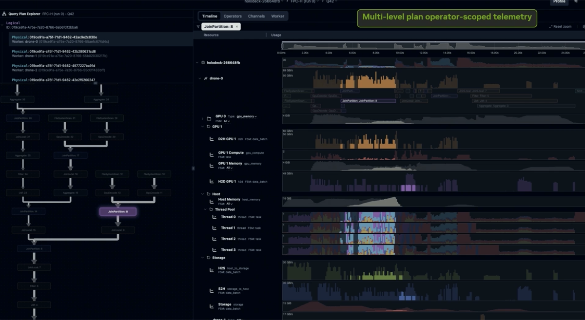
I’ll focus on the high-level algorithm libcudf uses to compute a simple Groupby + Sum aggregation on the GPU, taking you through its flow from the initialization of data structures to identifying unique groupings, and aggregating the data into final output buffers. Throughout, I’ll highlight the libcudf CUDA kernels used, how they take advantage of the GPU’s limited but very fast shared memory to update intermediate results in a massively parallel way, and use block synchronization to ensure threads remain in lockstep. I’ll also describe some of the other libraries libcudf relies on, such as cuCollections for the static sets and hashmaps, and the Thrust library for lower-level data-parallel algorithms like scatter and for_each. Future posts will provide a more in-depth look at an actual run of the algorithm and its performance, also introducing a new visualization tool I have developed to understand the flow of interaction between CPU and GPU.
2. Setup: Software and Hardware used
Library Versions
The investigation was performed on RAPIDS v26.02.00, released on February 4, 2026. The cuCollections dependency used is pinned to commit d3701ae.
The code examples in this post link to my own annotated forks that include additional comments to aid understanding:
GB10 Device
This analysis was performed on the DGX Spark running the GB10 NVIDIA GPU (Blackwell). Here are some key hardware specs relevant to this analysis to keep in mind:
| Spec | Value |
|---|
| Architecture | Blackwell (SM 12.1) |
| Streaming Multiprocessors | 48 SMs |
| CUDA cores | 6,144 (128 per SM) |
| Shared memory per SM | 100 KB (max per block: 99 KB) |
| L2 cache | 24 MB |
| Memory | 128 GB LPDDR5x, unified (CPU + GPU share the same pool, zero-copy via ATS) |
| Memory bandwidth | ~273–301 GB/s |
| Host CPU | 1× Grace (20-core Arm Neoverse V2) |
The unified memory architecture means there is no PCIe transfer step for the input table, the Arrow Parquet file is read directly into the shared pool and is immediately accessible by both CPU and GPU. The memory bandwidth figure (~273–301 GB/s) will be the primary bottleneck for this workload, as the hash-set initialization and Interlude scans are purely bandwidth-bound.
Code Invoked
The input dataset is the order table from TPCH with 100 million rows (1.8 GB Parquet file). Future posts will explore much larger datasets. The below libcudf C++ code is invoked on an ingested table stored in the Apache Arrow format:
// Assume Table already loaded into GPU memory
cudf::table_view tv = cudf_table->view();

// Create GroupBy operator by specifying the `key` column to group on
cudf::groupby::groupby gb(cudf::table_view{{tv.column(src.key_col)}});

// create aggregation for each column, here only 1 SUM agg
cudf::groupby::aggregation_request req;
req.values = tv.column(src.value_col);
req.aggregations.push_back(cudf::make_sum_aggregation<cudf::groupby_aggregation>());

// Aggregate on default stream
auto [result_keys, agg_results] = gb.aggregate({req});
The equivalent SQL command is:
SELECT   o_orderstatus,
         SUM(o_totalprice) AS total_price
FROM     orders
GROUP BY o_orderstatus;
The goals are:
- Understand how libcudf selects and executes the groupby sum path using a string key and float64 column.
- Break down the algorithm into understandable pieces and show where in the code these are implemented
- Identify the main GPU kernel launch to its source location in cuDF and associated libraries.
- Explain the two-level shared-memory aggregation strategy that libcudf uses to reduce global atomic contention.
In a followup post, I will cover the following:
- Capture a real run of the algorithm with real Nsight Systems on GB10: confirms kernel names, ordering, and timing on a 100M-row workload.
- Review each kernel performance with Nsight Compute
- Look at the flow of messages using a custom viewer I have developed.
With 100M input rows that need to be reduced into K distinct o_orderstatus values, a naïve GPU approach, one global atomic-add per row directly into the output column, will suffer from severe memory contention, particularly when cardinality is low. cuDF avoids this by staging the reduction through shared memory.
3. Architecture at a Glance: The Four-Phase Data Flow
The diagram below shows the overall execution of the aggregation from the GPU’s perspective (from left to right), covering kernels and main data structures used.
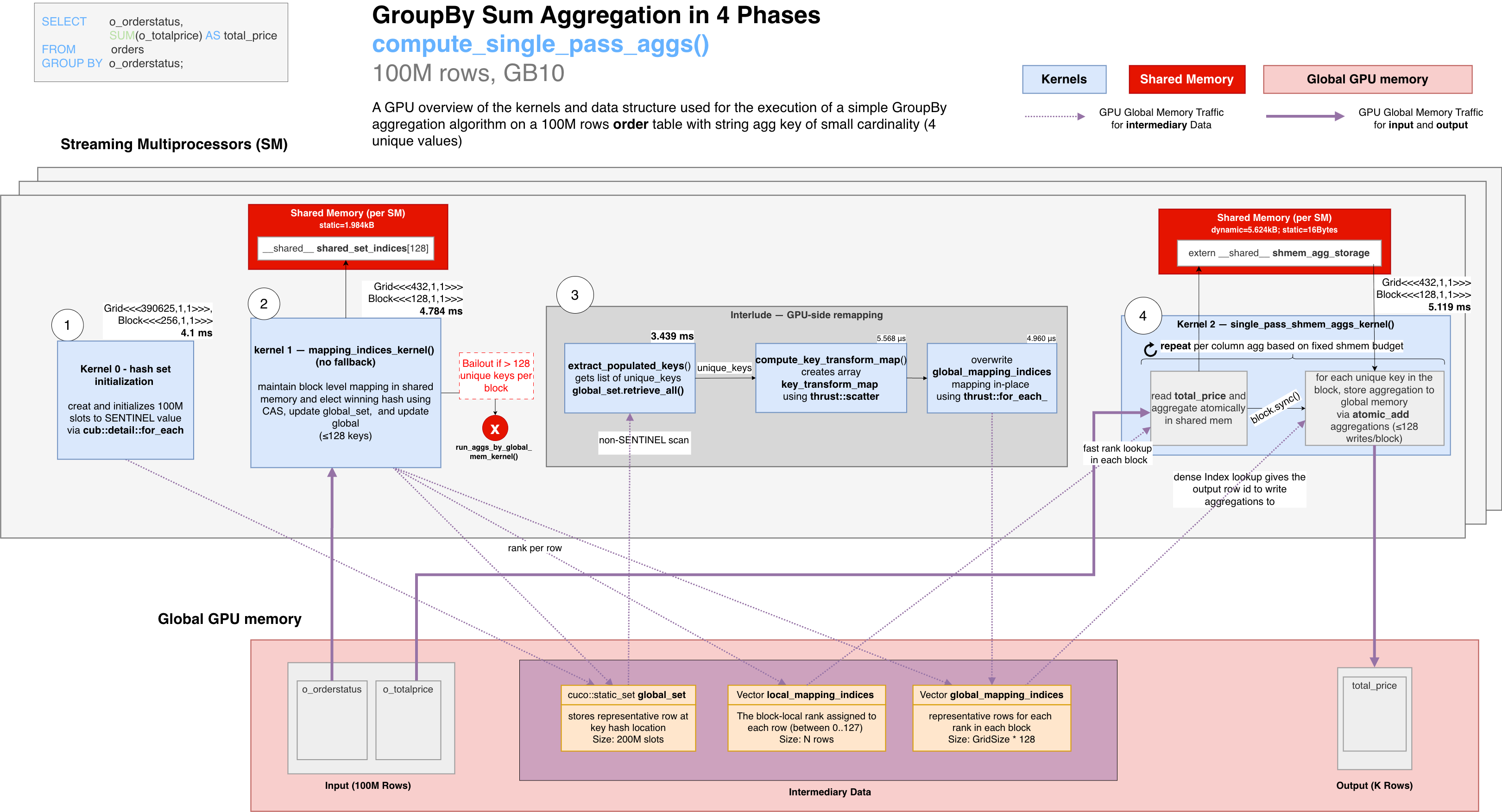
Use it as a map that links together all the details. The following sections below will zoom into each region: the kernel implementations (§5), and a step-by-step trace (§6), and more details about the global_set structure (§8)
Four algorithmic steps are highlighted:
- Initialization
- Block Level Membership and Index Mapping
- Interlude: Dense output index remapping
- Final step: Shared-memory accumulation + flush
The diagram highlights the different data structures stored in global memory and those in the shared memory, with reference to the 100M row dataset.
Global memory (visible to all blocks):
- Input:
o_orderstatus, o_totalprice (N=100M rows)
- Intermediary:
global_set (800 MB, 200M slots each 4 bytes), local_mapping_indices (one int32 per row), global_mapping_indices (128 int32 entries per block)
- Output:
total_price (K values)
Shared memory (private to each SM, discarded after the kernel):
shared_set / __shared__ slots[128]: phase 2 only; the cuco::static_set_ref hash map backing store, used by find_local_mapping to probe for key existence and assign block-local ranks via CASshared_set_indices[128]: phase 2 only; parallel flat array mapping each block-local rank to the first input row that claimed it (rank → representative row-index)shmem_agg_storage: phase 4 only; dynamic partial-sum accumulator storage indexed by block-local rank. For one double SUM over 128 ranks, the logical accumulator is 1 KB before alignment and any additional per-aggregation layout overhead.
4. The GroupBy.Sum() Algorithm
- Initialization:
- Before any row is processed, a global hash set (
global_set) is initialized to size 2x the input (200M slots) with a SENTINEL value (spawning a cub::detail::for_each on the gpu side).
global_set[0..200M) <- SENTINEL
- Block Level Membership and Index Mapping:
- This phase reads the key column and determines which
o_orderstatus group every input row belongs to. At this point the grouping is only local to a block. Each CUDA block uses a private hash table in shared-memory to map its rows to at most 128 distinct keys, assigning each a block-local rank (see below what is a block-local rank?).
- For each new key, using
CAS (the compare-and-swap atomic instruction), it atomically elects a single representative row where that key was first seen and inserts it into global_set to be used across all blocks.
- Two index arrays are maintained for use in later phases: 1) the
local_mapping_indices stores the block-local rank value allocated to each row later used to generate the per block aggregation, and 2) the global_mapping_indices stores the winning row for each rank slot of that block, later turned into a global ranking.
local_mapping_indices[row]        -> the block-local rank assigned to row
global_mapping_indices[blk*128+r] -> The representative row index for each rank slot in each block
global_set insert/find(rep_row)   -> The winning representative row at the key hash slot
- Interlude: Dense Output Index Remapping:
- Between the two main kernels, a set of device operations scans
global_set (via retrieve_all / cub::DeviceSelect::If) to collect the K representative row-indices, then builds a dense output ordering (0..K-1) via thrust::scatter, and rewrites global_mapping_indices in-place via thrust::for_each_n so every block agrees on the same output slot for each group. These algorithms launch over the full input or hash-set range even though only K ≪ N slots are populated, trading excess thread count for uniform, divergence-free execution that saturates memory bandwidth.
global_mapping_indices[blk*128+r] -> dense output index in total_price[0..K-1]
- Shared-Memory Accumulation + Global Reduction:
- Now that membership and output ordering are known, each block accumulates its assigned
o_totalprice values entirely within shared memory (no cross-block, no global atomics yet).
- Each block then flushes only up to 128 partial
o_totalprice sums to the correct output slot using the remapped global_mapping_indices, one atomic-add per distinct o_orderstatus value per block rather than one per row.
- For this dataset the number of global atomics is reduced by a factor of roughly
100M / (num_blocks × avg_labels_per_block) compared to the naïve approach.
- The logic is repeated based on the number of aggregation outputs to produce and available shared memory within a block
r = local_mapping_indices[row]
shmem_price_accum[r] += o_totalprice[row]
global_label_idx = global_mapping_indices[blk*128+r]
total_price[global_label_idx] += shmem_price_accum[r]
Note: Phase 2 and Phase 4 communicate through the index arrays produced by Phase 2 and rewritten by the Interlude; no inter-block GPU synchronisation is needed between Phase 2 and Phase 4.
What is a block-local rank?
- The key idea behind the fast path is that each CUDA block first locally deduplicates the keys among the rows it processes, then connects those per-block results to the final global output groups. This is done via block-local ranks.
- Each CUDA block assigns a small integer, starting from 0, to each distinct
o_orderstatus value the first time it is encountered among that block’s assigned rows. That integer is the block-local rank: a dense index into the block’s private shared-memory accumulator array. In the fast path, valid ranks are 0..127. This numbering is private to this block; another block may assign rank 0 to “O” or any other o_orderstatus.
- The Interlude phase converts the representative row-indices stored in
global_mapping_indices after Phase 2 into final dense global output indices (0..K-1), where K is the total number of unique keys across all rows. This ensures that all blocks agree on the same output slot for each group before phase 4 runs.
5. Deep Dive into each phase: Kernels and Data Structures
Now that the data flow and hash-set mechanics are established, this section revisits the same phases at the level of the actual kernels and helper functions. All the kernels below are invoked from a single host function, compute_single_pass_aggs().
Phase 1: Hash set initialization
Before any row is processed, a cub::detail::for_each kernel sweeps all 200M slots of global_set and writes the SENTINEL value (typically INT32_MAX) to each one. This establishes the “empty” state that insert_and_find’s CAS loop uses to distinguish occupied from free slots. At 4 bytes × 200M slots = 800 MB of writes, this kernel is purely memory-bandwidth-bound (~4.1 ms on this dataset).
Phase 2: Key insertion and index mapping
Every input row is processed by the mapping_indices_kernel kernel. For each row, the thread performs three steps:
-
Block-local deduplication: find_local_mapping() inserts the row’s key into shared_set, a block-private mini hash table cuco::static_set_ref backed by __shared__ slots[] (capacity = GROUPBY_CARDINALITY_THRESHOLD = 128 unique keys). shared_set is used only for existence checks (new key vs. duplicate); a separate flat __shared__ array shared_set_indices[rank] = row_idx maps each block-local rank to the first input row that claimed it. local_mapping_indices[row] is written with the block-local group rank (0..127): for a new key it is assigned by atomically incrementing cardinality; for a duplicate it is copied from local_mapping_indices[matched_row] after a block.sync(). local_mapping_indices provides a local per block grouping of the rows that will be re-used in phase 4 of the later accumulation step.
-
Global key registration: find_global_mapping() iterates over shared_set_indices[0..cardinality-1] and inserts each representative row-index into the global cuco::static_set. The CAS inside global_set.insert_and_find() atomically elects a single representative row for that key across all blocks. The winning row-index is stored in global_mapping_indices[block × 128 + rank]. Only one global insertion is made per distinct o_orderstatus value per block, not per row.
-
Overflow detection: if cardinality > 128, the needs_global_memory_fallback flag is set and all threads in the block break out of the input loop. After the kernel, the host checks this flag and if set, falls back a slower naïve global-memory aggregation path instead run_aggs_by_global_mem_kernel.
Phase 3, Interlude: Dense output index remapping
When there is no overflow, extract_populated_keys() is invoked to extract unique key row-indices from global_set into a contiguous buffer via cuco::static_set::retrieve_all(), which fires two CUB kernels (DeviceCompactInitKernel + DeviceSelectSweepKernel).
The key transition in this phase is the meaning of global_mapping_indices:
Before Interlude:
global_mapping_indices = representative input row-index, in range [0..N-1]
After Interlude:
global_mapping_indices = dense output index into total_price[], in range [0..K-1]
This is done in 2 steps:
- A
compute_key_transform_map() step builds the dense renumbering (key_transform_map) that maps any representative input row-index to a compact output slot [0, K):
key_transform_map[representative_input_row_idx]
     = output_group_index   (0..K-1)
- A second
thrust::for_each_n kernel then rewrites global_mapping_indices in place using this map so that every entry holds a finalized output group index.
Phase 4: Shared-memory accumulation + flush
This phase is implemented by a single kernel, single_pass_shmem_aggs_kernel
Each block declares extern __shared__ cuda::std::byte shmem_agg_storage[]: a dynamically-sized shared memory buffer laid out by calculate_columns_to_aggregate() as num_agg_columns × cardinality × sizeof(element_type) bytes (plus alignment padding), where cardinality ≤ GROUPBY_CARDINALITY_THRESHOLD = 128.
The kernel breaks the computation into a loop covering a number of aggregation output columns based on available shared memory, with the inner loop running the following two sub-phases:
┌─ Sub-phase 1: per-row accumulation into shared memory ──────────────────────┐
│  For each `row` assigned to a block, use previously generated               |
| `local_mapping_indices` to aggregated rows with same key in each block:     │
│    shmem_agg_storage[local_mapping_indices[row]] += source_value[row]       │
│    (via cudf::detail::atomic_add into shared memory)                        │
└─────────────────────────────────────────────────────────────────────────────┘
                              |
                          block.sync()
                              |
                              V
┌─ Sub-phase 2: flush partial results to global output columns ───────────────┐
│  For each `unique key` resident in this block:                              │
│    target_global_col[global_mapping_indices[blk×128+rank]]                  │
│        += shmem_agg_storage[rank]                                           │
│    (via cudf::detail::atomic_add into global memory)                        │
└─────────────────────────────────────────────────────────────────────────────┘
target_global_col will contain the final aggregation value for each column.
The global atomic_add in sub-phase 2 is reached via an inlined two-level compile-time template dispatch (type_dispatcher × aggregation_dispatcher) that resolves the runtime column type and aggregation kind to a single pre-compiled specialization with no GPU branching. For SUM on double input (o_totalprice), this lands at update_target_element_gmem<double, SUM>, which calls cudf::detail::atomic_add directly.
Wrapup: Output Key Gather
After aggregation, the unique key row-indices retrieved from the hash set are used to gather the corresponding rows from the original input keys table into a dense output keys table:
output_keys[i] = input_keys[unique_key_indices[i]] for i in [0, K)
For string key columns this gather requires a multi-step CUB prefix scan over character offsets followed by a parallel character copy kernel (gather_chars_fn_char_parallel).
The example below traces the whole algorithm with two small blocks. The values are artificial, but the roles of local_mapping_indices, global_mapping_indices, unique_key_indices, and key_transform_map match the real execution.
Setup:
- 2 blocks (B0, B1),
GROUPBY_CARDINALITY_THRESHOLD = 128- K=3 unique aggregation key values,
"F", "O", and "P"
- MurmurHash3 slot assignments in the 200M-slot
global_set:
hash("F")%200M = 47_000_000hash("O")%200M = 103_000_000hash("P")%200M = 182_000_000.
Each block is assigned a contiguous slice of the 100M input rows:
Block0 (rows 1000..1004):
| Row | Key |
|---|
| 1000 | "F" |
| 1001 | "O" |
| 1002 | "F" |
| 1003 | "P" |
| 1004 | "O" |
Block1 (rows 5000..5004):
| Row | Key |
|---|
| 5000 | "O" |
| 5001 | "P" |
| 5002 | "O" |
| 5003 | "F" |
| 5004 | "P" |
Step 2: Phase 2 block-local rank assignment + global set insertion (compute_mapping_indices)
- Each block builds a private shmem hash set, assigning a
rank to each new key on first encounter.
- For every key that is new to that block, it calls
insert_and_find(row_idx) on the shared global_set (200M slots, cuda::thread_scope_device) to claim a globally unique slot via CAS.
insert_and_find returns {iterator_to_slot, bool_inserted}.- Dereferencing the iterator (
*it) yields the row index stored in that slot; always the winning thread’s row_idx, regardless of which thread won the CAS race.
- That row index is what gets written to
global_mapping_indices.
Assume Block0 wins the global CAS races, and each block assigns local ranks in first-seen row order. local_mapping_indices maps each input row to its block-local rank:
- Block0 first sees “F”, then “O”, then “P” → F=rank0, O=rank1, P=rank2
- Block1 first sees “O”, then “P”, then “F” → O=rank0, P=rank1, F=rank2
local_mapping_indices: block-local rank per row:
| Row | Value | Description |
|---|
| 1000 | 0 | "F" → rank 0 (first seen) - Block0 |
| 1001 | 1 | "O" → rank 1 |
| 1002 | 0 | "F" duplicate → rank 0 |
| 1003 | 2 | "P" → rank 2 |
| 1004 | 1 | "O" duplicate → rank 1 |
| ... | | |
| 5000 | 0 | "O" → rank 0 (first seen) - Block1 |
| 5001 | 1 | "P" → rank 1 |
| 5002 | 0 | "O" duplicate → rank 0 |
| 5003 | 2 | "F" → rank 2 |
| 5004 | 1 | "P" duplicate → rank 1 |
| .. | | |
| N-1 | | |
global_set after Phase 2 (200M slots, only 3 occupied), stores the winning representative row for this key, all from Block0 rows.
| Slot | Value | Description |
|---|
| hash("F") % 200M | 1000 | First winning row with key "F" |
| hash("O") % 200M | 1001 | First winning row with key "O" |
| hash("P") % 200M | 1003 | First winning row with key "P" |
| all other ~199M slots | SENTINEL | Empty |
global_mapping_indices after Phase 2 contains representative input row indices, not yet mapped to the dense output grouping. Since B0 won the CAS races, B0’s winning rows are what gets stored:
| Index | Value | Description |
|---|
| [0×128 + 0] | 1000 | B0 rank 0 ("F") → winning row 1000 |
| [0×128 + 1] | 1001 | B0 rank 1 ("O") → winning row 1001 |
| [0×128 + 2] | 1003 | B0 rank 2 ("P") → winning row 1003 |
| [0×128 + 3..127] | SENTINEL | Unused B0 slots |
| [1×128 + 0] | 1001 | B1 rank 0 ("O") → uses B0 winning row 1001 |
| [1×128 + 1] | 1003 | B1 rank 1 ("P") → uses B0 winning row 1003 |
| [1×128 + 2] | 1000 | B1 rank 2 ("F") → uses B0 winning row 1000 |
| [1×128 + 3..127] | SENTINEL | Unused B1 slots |
| .. | SENTINEL | Unused |
| NBLOCKS * 128 - 1 | SENTINEL | Unused |
Note: B1 also attempted to insert “O”, “P”, and “F” but the CAS returned DUPLICATE. The iterator still points to the existing slot, so *it gives the same row index B0 stored. Both blocks therefore agree on the same representative input row index per key.
retrieve_all() scans global_set linearly from slot 0 to slot 199M via cub::DeviceSelect::If, collecting the row-index values stored in each non-SENTINEL slot:
scan order: slot hash("F")%200M comes first, then hash("O")%200M, then hash("P")%200M
            (i.e. in ascending slot-position order, regardless of insertion order)

unique_key_indices = [1000, 1001, 1003]   ← representative input row index per slot, in slot-scan order
                       i=0    i=1    i=2
These are the same row indices already in global_mapping_indices, just deduplicated by scanning the hash table. Their position in unique_key_indices (0, 1, 2) defines the dense output row each key will occupy.
Scatters counting values 0, 1, 2 to positions unique_key_indices[0,1,2]. The result is an array of size N (number of input rows), where each populated index is the representative input row index mapped to its final dense output row.
| Index | Value | Description |
|---|
| [1000] | 0 | Row 1000 ("F") → dense output row 0 |
| [1001] | 1 | Row 1001 ("O") → dense output row 1 |
| [1002] | - | - |
| [1003] | 2 | Row 1003 ("P") → dense output row 2 |
| all other ~99M entries | (uninitialized) | Irrelevant; never read |
Step 5: thrust::for_each_n: rewrites global_mapping_indices in-place with dense output rows
Each non-SENTINEL entry (a representative input row index in 0..N-1) is replaced with key_transform_map[old_idx] (the corresponding dense output row in 0..K-1). The representative rows 1000, 1001, and 1003 are not usable as output indices directly; there are only K=3 output rows, so they must be remapped to 0, 1, and 2:
global_mapping_indices after remapping (dense output indices, replacing representative row indices): Notice that the ranks have the same value across all blocks; it is a global mapping.
| Index | Value | Description |
|---|
| [0×128 + 0] | 0 | B0 rank 0 ("F") → output row 0 |
| [0×128 + 1] | 1 | B0 rank 1 ("O") → output row 1 |
| [0×128 + 2] | 2 | B0 rank 2 ("P") → output row 2 |
| [0×128 + 3..127] | SENTINEL | Unused B0 slots |
| [1×128 + 0] | 1 | B1 rank 0 ("O") → output row 1 |
| [1×128 + 1] | 2 | B1 rank 1 ("P") → output row 2 |
| [1×128 + 2] | 0 | B1 rank 2 ("F") → output row 0 |
| [1×128 + 3..127] | SENTINEL | Unused B1 slots |
| .. | SENTINEL | Unused |
| NBLOCKS * 128 - 1 | SENTINEL | Unused |
Now we have a mapping from every row to its block-local accumulator, and from every block-local accumulator to its global output row. Each block reads its rows, accumulates o_totalprice into shmem using local_mapping_indices[row] as the shmem slot, then flushes at most 128 partial sums to global memory using global_mapping_indices[block*128 + local_rank] as the total_price output index.
7. Algorithm Complexity Summary
Assuming the following:
- N = total number of input rows (100M in this dataset).
- K = number of distinct groupby keys.
- capacity = hash-table size (2N slots = 200M).
| Stage | Time complexity | Dominant cost |
|---|
| Phase 1: hash set init | O(N) | Memory bandwidth: write sentinel to 2N slots (~4.1 ms) |
| Phase 2: key insertion + local mapping | O(N) avg | Hash probing + atomic inserts |
| Phase 3 Interlude: unique key extraction + dense index remap | O(capacity) = O(2N) | NOT O(K), retrieve_all() must scan every one of the 200M hash-table slots to find the K occupied ones. Cost is fixed by table size, not by the number of distinct keys (~3.4 ms even when K=3) |
| Phase 4: SUM accumulation | O(N) | Shared-memory atomics (fast) + global atomics (flush) |
| Key gather | O(K + total key bytes) for strings | Offset scan + character copy |
Total: O(N) average with low constant factors when cardinality ≤ 128 groups per block. The asymptotic result is simple; the practical win comes from changing global atomic frequency from per-row to per-block-per-group.
8. Appendix: A Deeper Look into hash set global_set
The hash groupby is built around a device-side open-addressing hash set (cuco::static_set), referred to as global_set in the code, that stores one representative input row-index per unique key. It does not store the aggregation key values directly; instead, each stored row-index points back into the original key column, and the row hasher/comparator use that row to hash and compare the key value.
Since many rows can have the same aggregation key, insert_and_find() uses CAS (compare-and-swap) to claim empty global slots and elect one representative row for each key across all blocks. Each block first maintains its own block-private shared_set in shared memory to deduplicate rows locally, then only the block-local representative rows are inserted/looked up in global_set.
Multiple blocks may attempt to register the same key, but only the first successful CAS writes that key’s global representative row-index into the set. In order to minimize collision cost without knowing the distinct key count in advance, the set’s capacity is sized for the worst case in which every input row has a distinct key: twice the number of rows in the dataset.
global_set slot layout:
- N = 100M rows
- load factor = 50%
- capacity = 2 × num_input_rows = 200M slots
Example content with 2 unique key values:
| # | value | Notes |
|---|
| 0 | EMPTY | |
| 1 | EMPTY | |
| 2 | 7 | Row 7 has a unique o_orderstatus value that hashes into this slot |
| 3 | EMPTY | |
| … | … | |
| 1000 | 12 | Row 12 has a different unique o_orderstatus value that hashes into a different slot in this set |
| … | EMPTY | |
| 199M | EMPTY | |
Set design
The hash set is constructed in compute_groupby() with the following specifications:
- Key type:
int32_t (cuDF size_type). Row hashing and equality comparison are performed by cuDF’s row comparator against the o_orderstatus (utf8) column. MurmurHash3 over character bytes, byte-wise equality.
- Capacity:
2 × N slots where N = num_input_rows (used as a worst-case upper bound for distinct key count; CUCO_DESIRED_LOAD_FACTOR = 0.5). For N = 100M rows: 200M slots × 4 bytes = 800 MB. Construction fires cub::detail::for_each::static_kernel<initialize_functor<long,int>> to fill all slots with the sentinel in parallel. For 100M rows, initialization costs 4.105 ms, ~23.5% of total groupby kernel time.
- Probing scheme:
cuco::linear_probing<1, row_hasher_with_cache_t>. Linear probing with CGSize=1 (each probe step is handled by a single thread, advancing one slot at a time), with an optional row-hash cache (pre-computed hashes stored in a device_uvector).
- Thread scope:
cuda::thread_scope_device. All GPU threads can access the same set.
- Sentinel:
CUDF_SIZE_TYPE_SENTINEL = INT32_MAX. Marks empty slots.
- Memory:
rmm::mr::polymorphic_allocator. Backed by the caller-supplied RMM pool.
- Storage layout:
cuco::storage<BucketSize=1>. Two-level slot hierarchy: array of buckets, each holding BucketSize contiguous slots. BucketSize > 1 lets a thread probe multiple slots per step (beneficial for memory-bandwidth-bound workloads). For cuDF GroupBy, hardcoded to GROUPBY_BUCKET_SIZE = 1 (flat per-slot probing); appropriate here since key cardinality is low and contention is minimal.
Finding/Inserting a key in the set
The set stores row indices (int32_t), not actual key values. When the set needs to hash or compare a candidate slot, it calls back into the original input column data on the GPU (via d_row_hash). This indirection is set up before any kernels run, in dispatch_groupby():
preprocessed_table::create(keys, stream): copies the column_device_view metadata structs (data pointers, null masks, type IDs) into a GPU buffer so kernels can dereference them. The actual column bytes were already in GPU memory via RMM. Cost: ~143 bytes (one string column’s metadata, as seen in the RMM trace).self_comparator: host factory that wraps the preprocessed_table and produces device_row_comparator, a GPU callable implementing operator()(i, j) → byte-wise string equality via type_dispatcher.row_hasher: same pattern; produces device_row_hasher, a GPU callable implementing operator()(i) → MurmurHash3 over all columns of row i. Both share the same preprocessed_table via shared_ptr to avoid a redundant GPU upload.
These two callables are then embedded directly into the cuco::static_set constructor as the probing scheme and equality comparator, so every insert and lookup the set performs reaches back into the original key column memory.
insert_and_find(i) logic for row index i:
1. slot = d_row_hash(i) % 200M_slots          ← initial probe position from o_orderstatus string bytes

2. occupant = *slot
  pre-CAS check: d_row_equal(i, occupant)    ← does the row stored in this slot match row i's key?
      EQUAL     → return {slot, false}         ← key seen before; occupant is the representative (no CAS needed)
      AVAILABLE → go to step 3                 ← slot is empty (SENTINEL); attempt insert
      UNEQUAL   → slot += 1, repeat step 2    ← occupied by a different key; linear probe

3. CAS(slot, SENTINEL, i)                     ← atomically try to claim this empty slot
      SUCCESS   → return {slot, true}          ← we won; row i is now the representative
      DUPLICATE → return {slot, false}         ← another thread won the same key; slot holds the representative
      CONTINUE  → repeat step 2 at same slot  ← a different key raced us here; re-probe from this slot
Phase 2 kernel mapping_indices_kernel uses this operation in two scopes. First, each row probes the block-private shared_set to get a block-local rank. Then only the rows that represent keys new to that block probe the global global_set, where the CAS in step 3 performs the cross-block election: whichever thread wins the compare-and-swap for a given o_orderstatus value becomes the globally agreed representative row for that key. The CONTINUE result (a raced-but-different-key loss) sends the thread back to re-evaluate the slot it just lost, not to advance, since the winner may have written a key equal to i.
]]>
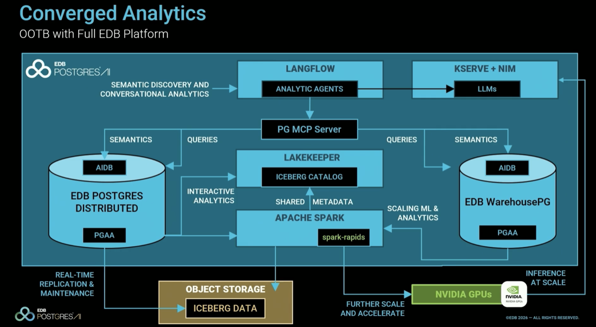


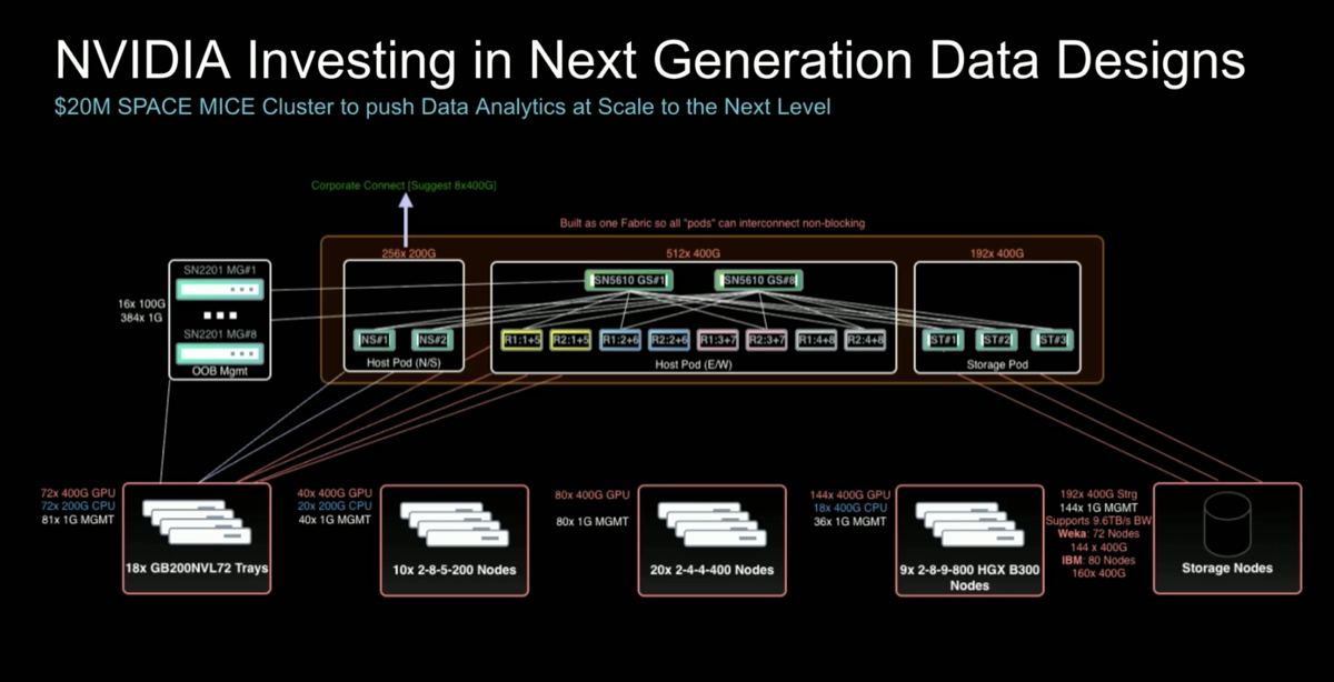
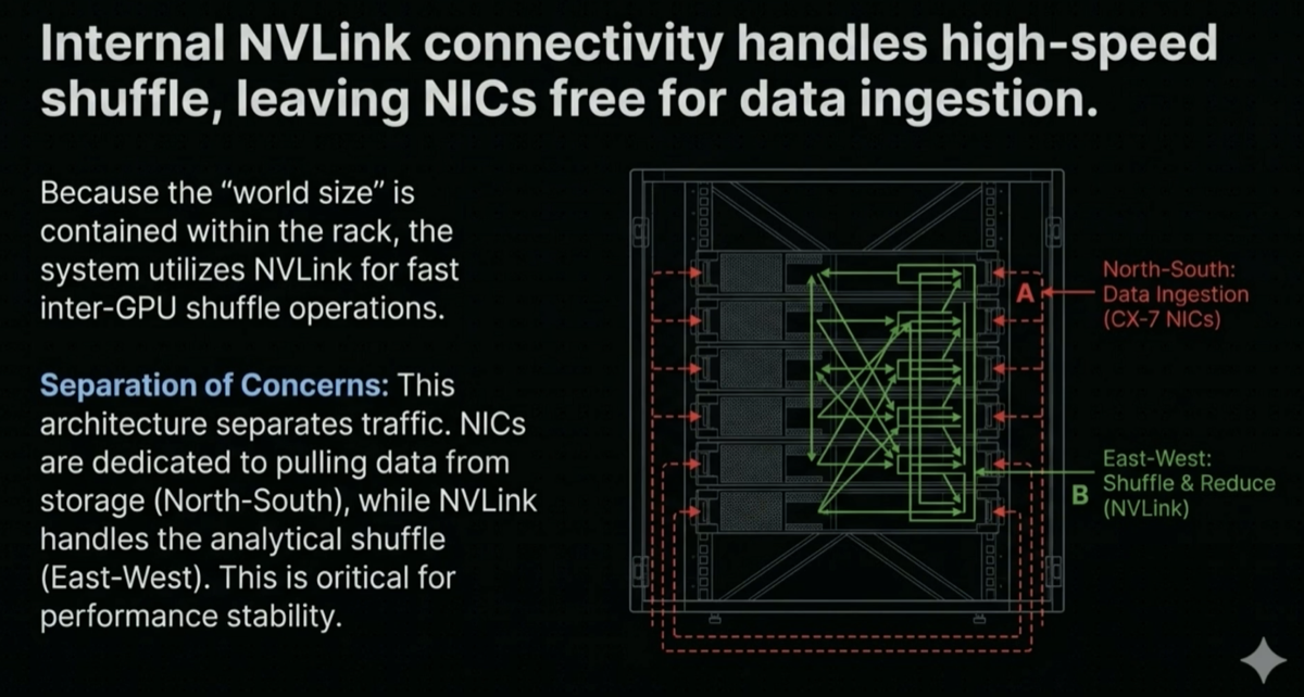

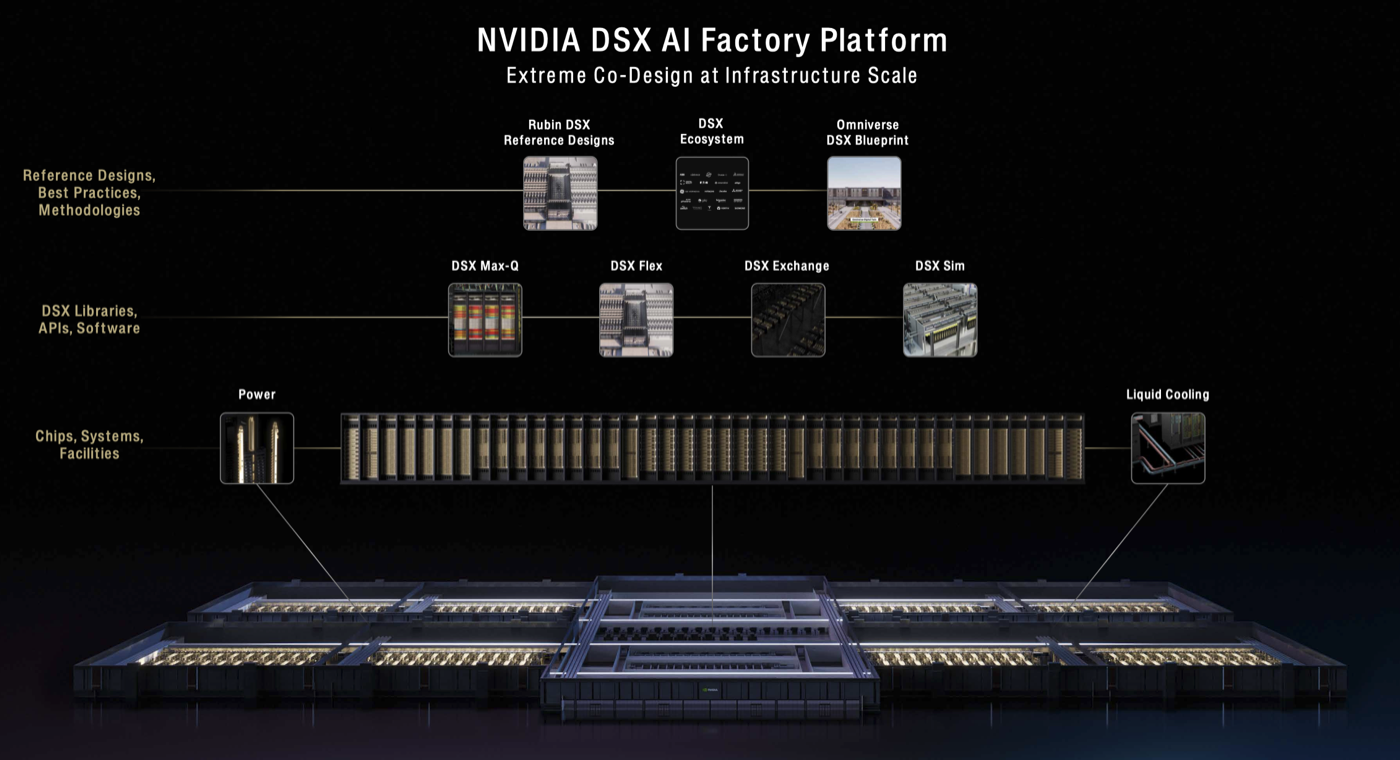 The video summarizes all the components of the DSX AI factory platform